As a bit of a side project at work recently, I did some modeling work on TESS, which is a NASA spacecraft that was launched to help search for exoplanets using the transit method (I know, you could never have guessed that from the name’s acronym breakdown). Working with satellites as much as I do, this was a really interesting project, because it was quite distinctive in its orbit and mission architecture from most spacecraft that I get to study on a regular basis. For one thing, it is a remarkably low-cost, robust, straightforward system, quite different from what you often see with NASA programs, which because of their scientific goals are often pushing the very edge of our capabilities and therefore become very complex and very expensive. For another, it utilizes a simply fascinating orbit. Since I’ve been trying to post occasional in-depth articles on various academic topics, it seemed appropriate to share some of what I learned from that project here.
There are a lot of directions I could take this post, and it would be very easy to get mired in complexity, but since I have no way of knowing how much background you, as the reader, might have on the subjects covered herein, I’m going to break the post into two parts, and try to explain everything to the most approachable extent that I can. That being said, if you are left confused about anything in the post, or have any additional questions, or simply want more detail than I shall be herein providing, I encourage you to ask, either in the comments below, or through the site’s contact form, and I would be more than happy to provide what answers I might have (please note: my spam filters block anything with a link). To get started, let’s talk about exoplanets.
Exoplanets
It wasn’t that long ago, maybe a century or so, that we thought that our galaxy comprised the entire universe. When science fiction icons like Star Trek and Star Wars first came out, no one knew how common stars with planetary systems might be, or even if they existed at all; the first definite exoplanets (planets orbiting other stars) weren’t discovered until the mid-1990s. In fact, there were many astronomers and astrophysicists before and even after that time who thought that planetary systems might well be an anomaly, and that the majority of stars would be barren. We have since found that the opposite is true; it seems that the majority of stars have at least some kind of planetary system, even if most are nothing like that of our own star with which we are familiar. We’ve gone in the course of a decade or two from questioning the very existence of planets, to having confirmed the existence of thousands of exoplanets, and that is simply remarkable.
An exoplanet is simply any planet orbiting another star, and they can take a staggering diversity of forms. The most common are probably so-called hot Jupiters, which are gas giants with mass comparable to that of Jupiter, but which orbit much closer to their host star, and often have some internal heat generation, besides (although the exact dynamics are as yet unknown). Other common exoplanets are called super-Earths, which are thought to be terrestrial in character like the Earth, but are significantly more massive. That being said, we’ve found everything in between, and to the extremes, besides, even including Earth-like planets in the so-called habitable zone (the range from a star in which a water cycle could be reasonably propagated). It is worth noting with all of these comparisons that there is significant bias in terms of what types of planets are most readily detectable with our current sensors, which is what we’ll talk about next.
There are five major methods currently being used to find and confirm the existence of exoplanets: radial velocity, transit, direct imaging, gravitational microlensing, and astrometry. Of these, the most common are by far radial velocity and the transit method, while the other three have only been used a handful of times. In fact, the transit method has been used to detect more than three times as many exoplanets as the radial velocity method. However, I’ll give at least a brief description of all five of these techniques.
Radial Velocity
Also called the wobble method, this technique involves the gravitational interactions between a star and its planet. Stars are not fixed in space, and planets do not simply orbit around a star; the star also “orbits” around the planet. What’s really happening is that they are both orbiting around a mutual center of gravity, but that center is often so close to the center of the parent star (since the star is so much more massive than the planet) that it is barely perceptible. Fortunately, we the ability to measure the way the light emitted from a star changes based on the tiny wobble induced by the presence of a planet in orbit. This can allow us to infer the existence of a body orbiting a star.
Transit Method
This is by far the most common method, and it is besides the most intuitive (it’s also what TESS uses, logically enough). We can establish a light profile for a star through observing it over a period of time, and if that light profile dims in a periodic fashion, then we can infer that a planet is crossing between us and the star; think of it as detecting a planet by measuring its shadow.
Direct Imaging
I know I just said the transit method might be the most intuitive, but you might argue that direct imaging is the most intuitive, since this is really just taking a picture of the exoplanet. However, it is extremely challenging to implement. Imagine trying to take a picture that can resolve the surface of a grain of sand with a camera on the moon – that might get you close to the difficulty of directly resolving a planet orbiting a distant star. Until you start working with these distances on a regular basis, it is difficult to fathom just how massive a distance even a single lightyear is.
Gravitational Microlensing
You may have seen headlines in the past few years about a phenomenon known as gravitational lensing. This is probably the most complicated of all of the detection methods, and to really understand what is going on here requires a comprehension of both electromagnetism and general relativity. However, I will do my best to explain it without getting too technical. We know from experience that light waves are bent by passage through a medium, and this is how a lens works, whether that’s a magnifying glass or your eyeglasses (or, for that matter, your eyes). Additionally, relativity informs us that massive objects distort the fabric of spacetime, and that this is the means by which gravitational force is communicated.
It turns out that electromagnetic rays (lightwaves) are also bent by this curvature of spacetime, which can result in the same kinds of distortions and magnifications that are the result of lightwaves passing through a physical medium. This is the phenomenon known as gravitational lensing. So when lightwaves from a distant source pass by a massive object, like a star, on their way to our detectors here on Earth, they are distorted in a predictable way, and we can measure that distortion and understand things both about the original source of the lightwaves, and the massive entity that distorted them.
The gravitational microlensing technique for exoplanet detection measures very small-scale distortions of lightwaves from stars resulting from the gravitational presence of orbiting planets. These disturbances are tiny, which is why we’ve detected relatively few exoplanets using this method, but unlike the other methods this technique does not require as specific of an alignment between the Earth, the exoplanet, and the host star.
Astrometry
While the other names fairly succinctly describe the techniques involved, astrometry is just a generic term of the measurement of anything in astronomy, usually the relationships between stars. Not so long ago, we thought that stars were relatively fixed in space, and though we have since found that to not be the case, the movements they do make relative to us are very small. It turns out that the presence of exoplanets around a star can affect its course enough to discernibly alter its relative motion with respect to Earth observatories, and we can measure and characterize those effects to determine the presence of planets. This technique has only led so far to the discovery of a single exoplanet, so I wouldn’t spend too much time pondering it; focus instead on the transit method, the radial velocity (wobble) method, and the direct imaging method.
Orbit
Orbits are chosen based on mission requirements and capabilities. In the case of TESS, the mission required a dynamically stable orbit with a perigee (point of closest approach to the Earth) above GEO (the altitude at which a satellite appears to hover in place over a particular location on the Earth’s surface), and because of the spacecraft’s limitations, it could not require significant station-keeping or other on-orbit maneuvering. To break that down, it needed an orbit that was easy to get into, that didn’t change too much in the long term (2-4 years), and that at its closest point was at least ~40000 km from the Earth.
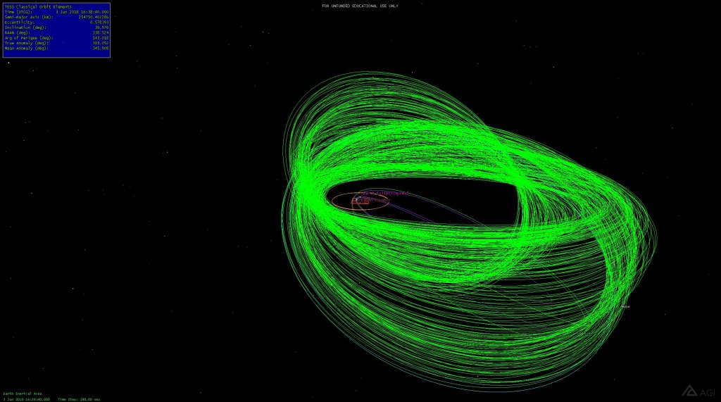
For the purpose, they chose something called a P/2 lunar resonance orbit. In this orbit, the apogee is just shy of the moon’s orbit, and the perigee is above GEO (as required), which gives it a period (the time it takes to complete one full orbit) that is exactly half that of the moon (about 13.8 days). As a result, the moon’s gravitational influence on the orbit will be balanced out, coming from opposite directions, over the course of a month, which satisfies the dynamically stable requirement. In order to achieve such an orbit in an efficient fashion, a series of phasing orbits, including a lunar injection orbit, are used, which I’ve shown in these graphics (the green circle around the Earth represents the GEO belt):
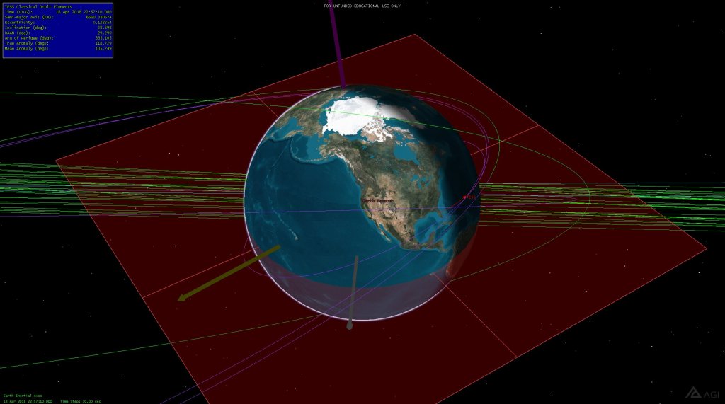
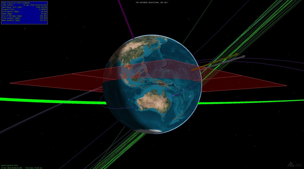

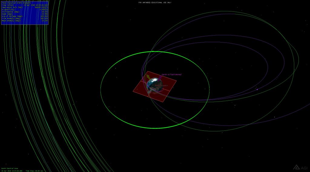
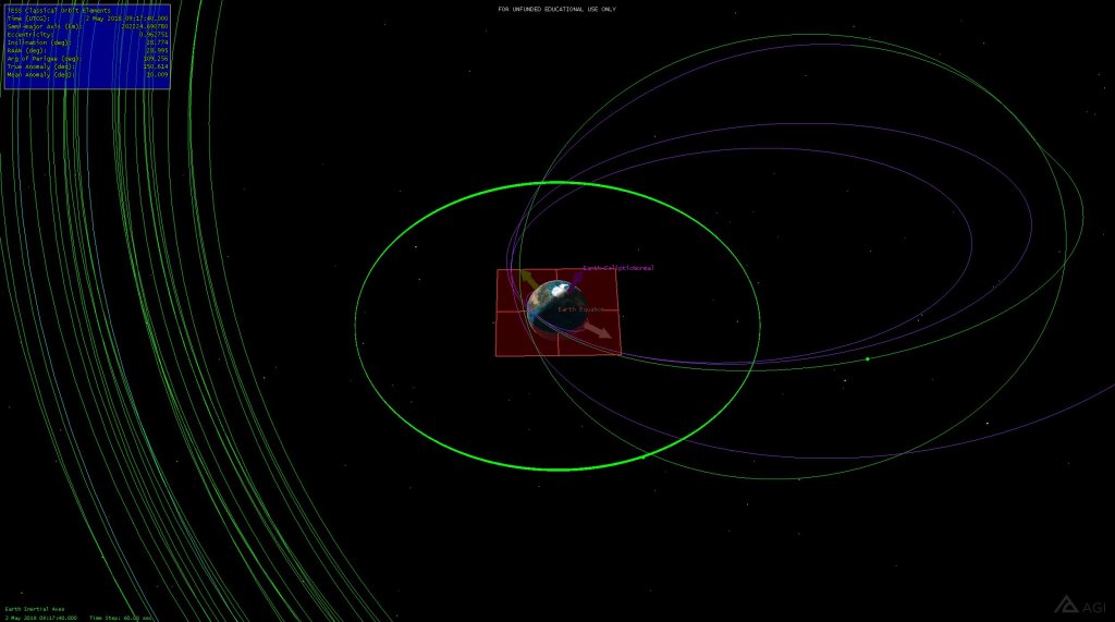
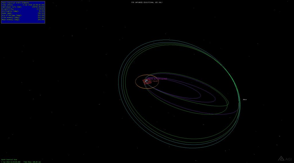
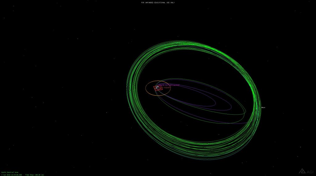
This orbit is simply fascinating. You can see in these next images how it changes over the course of two months, a year, four years, and twelve years. It clearly remains dynamically stable over several years, though it begins to drift significantly after twelve (although I believe it still meets the mission requirements). The models I’ve generated here appear similar to other models generated by the TESS team, so I’m fairly confident in what I came up with for this project.


I hope that you found this interesting. There’s no real tie-in to writing for this post, although I suppose if you’re writing realistic science fiction it could be useful to understand orbits and exoplanets and detection methods. There is so much more that we could discuss on these topics, so if you have questions or would like to see more posts like this that go into more detail on these or similar concepts, please consider commenting below the post. If you want to learn more about how these simulations were generated, you can check out Astrogator Guild.

12 thoughts on “TESS: Transiting Exoplanet Survey Satellite”